Spreadsheets are powerful for organizing information, but finding and pulling the right data can take time without the right tools. That’s where VLOOKUP, HLOOKUP, and XLOOKUP come in. These lookup functions in Excel and Google Sheets make it simple to search through rows and columns and return exactly what you need. In this guide, you’ll see how each one works, learn practical examples, and pick up a few tips to use them more confidently.
Quick Comparison: VLOOKUP vs HLOOKUP vs XLOOKUP
| VLOOKUP | HLOOKUP | XLOOKUP | |
|---|---|---|---|
| Search direction | Down (vertical) | Across (horizontal) | Any direction |
| Return column/row | Must be to the right of the lookup column | Must be below the lookup row | Any position, any range |
| Multiple results | No | No | Yes (multi-column/row) |
| Default match | Approximate (TRUE) | Approximate (TRUE) | Exact (0) |
| Not-found handling | Returns #N/A (wrap in IFERROR) | Returns #N/A (wrap in IFERROR) | Built-in if_not_found parameter |
| Wildcard search | Yes (with approximate match off) | Yes (with approximate match off) | Yes (match_mode 2) |
| Excel compatibility | All versions | All versions | Excel 2021+ / Microsoft 365 |
| Google Sheets | Yes | Yes | Yes (since 2022) |
| Best for | Vertical tables where the lookup column is first | Horizontal tables where the lookup row is first | Any layout, especially when you need flexibility |
Each function is explained in detail below, with syntax breakdowns and step-by-step examples.
Understanding VLOOKUP
What is VLOOKUP?
VLOOKUP (or Vertical Lookup) is one of the most widely used functions in Excel and Google Sheets. It helps you find a value in a table by looking it up – vertically. It searches down the first column to find a match, then returning a value from the same row in another column.
How VLOOKUP Works (Syntax explained)
The VLOOKUP function follows this syntax:
=VLOOKUP(lookup_value, table_array, column_index_num, [range_lookup]) - lookup_value: The value that you want to match or find. VLOOKUP is case-insensitive
- table_array: The range of cells that contains your data
- column_index_num: The index of the column to return the value of. The leftmost column of your table_array is index 1.
- range_lookup: Optional. Enter FALSE for an exact match, or TRUE for an approximate match. This parameter may be omitted, in which case approximate matching is used
- Use FALSE in most situations where you require exact matches (such as looking up emails or IDs). TRUE is suitable mainly for numerical ranges (such as tax brackets or grades)
For more detailed information, visit Microsoft’s official VLOOKUP documentation.
Step-by-step VLOOKUP
Here’s how to use VLOOKUP, step-by-step.
1. Prepare your data
First, you should prepare a rectangular area in your spreadsheet with your data. Each row in the area should represent a single row of data.
- Make sure your data has clear column headers
- Ensure that the value you want to look up is in the first column of the range
- If using an approximate match, sort the first column in ascending order
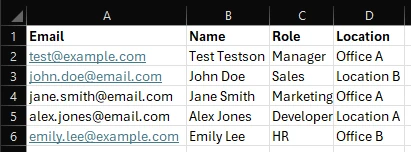
Example: You prepare an area where the first column is an email address, the second column a name, the third column a role, and the fourth column a location.
2. Identify what you want to find
Decide what you are searching for and which column has the result that you need.
- Remember that the first column, that contains your lookup value, has index 1
Example: You are looking for the role, which is the column with index 3.
3. Write the VLOOKUP formula
Click into the cell where you want the result. Type =VLOOKUP( and enter:
- the lookup value (e.g. a cell reference or text in quotes)
- the table range (e.g. an area or a named range)
- the column index number
- FALSE for an exact match or TRUE for an approximate match
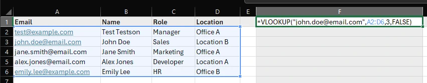
Example: In the cell F1, we type =VLOOKUP(“john.doe@email.com”, A2:D6, 3, FALSE)
VLOOKUP in practice
One of the many use-cases for VLOOKUP is item information lookup – the user chooses an item in a dropdown, and VLOOKUP finds the item’s price, weight, favorite color, or anything else.
Many Molnify users make use of VLOOKUP for data lookup. For an example of VLOOKUP fetching item information, see an example sales quote application.
Understanding HLOOKUP
What is HLOOKUP?
When your data is arranged in rows instead of columns, VLOOKUP isn’t always the best tool for the job. That’s where HLOOKUP — or Horizontal Lookup — comes in. It works just like VLOOKUP, but searches across the top row and returns values from rows below.
How HLOOKUP Works (Syntax explained)
The HLOOKUP function follows a syntax very similar to VLOOKUP:
=HLOOKUP(lookup_value, table_array, row_index_num, [range_lookup]) - lookup_value: The value that you want to match or find. HLOOKUP ignores case when comparing values
- table_array: The range of cells that contains your data
- row_index_num: The index of the row to return the value of. The topmost row of your table_array is index 1.
- range_lookup: Optional. Enter FALSE for an exact match, or TRUE for an approximate match. This parameter may be omitted, in which case approximate matching is used
- Use FALSE in most situations where you require exact matches (such as looking up emails or IDs). TRUE is suitable mainly for numerical ranges (such as tax brackets or grades).
For more details, see Microsoft’s official HLOOKUP documentation.
Step-by-step HLOOKUP
Here’s how to set up HLOOKUP, step by step.
1. Organize your data
Prepare an area for your data, so that each column represents a row of data
- Make sure your data has clear row headers
- Ensure that the value you want to look up is in the first row of the range
- If using an approximate match, sort the first row in ascending order
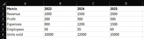
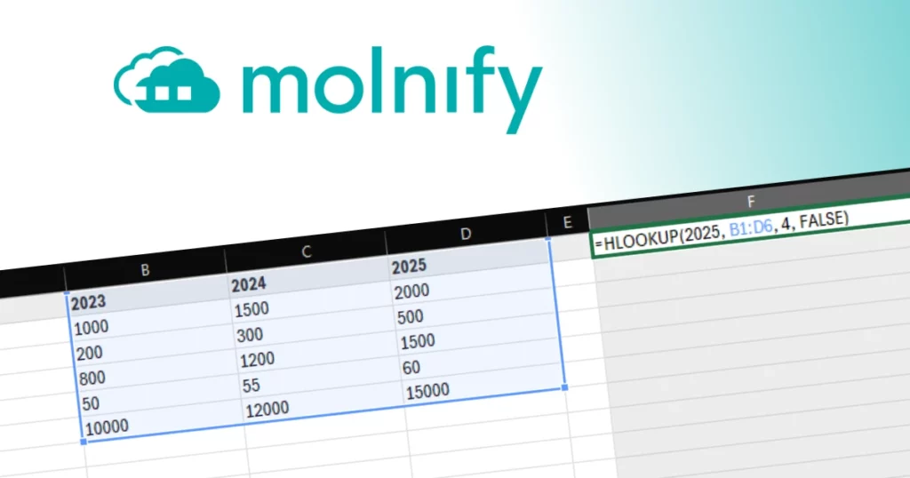
Example: You have financial data per year. Each column corresponds to a year, and the rows are, in order: Revenue, Profit, Expenses, Employees, and Units sold.
2. Identify what you want to find
Decide what you are searching for and which row has the result that you need.
- Remember that the first row, that contains your lookup value, has index 1
Example: To find the number of employees, we look up the row with index 4.
3. Write the HLOOKUP formula
Click into the cell where you want the result. Type =HLOOKUP( and enter:
- the lookup value (e.g. a cell reference or text in quotes)
- the table range (e.g. an area or a named range)
- the row index number
- FALSE for an exact match or TRUE for an approximate match
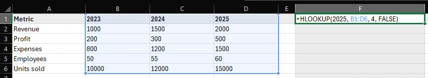
Example: In the cell F1, we type =HLOOKUP(2025, B1:D6, 4, FALSE)
Understanding XLOOKUP
What is XLOOKUP?
XLOOKUP, or Cross Lookup, is a newer, more flexible lookup function available in modern versions of Excel and in Google Sheets. Unlike VLOOKUP and HLOOKUP, which require you to choose between looking horizontally or vertically, XLOOKUP works in both directions. It searches a range for a match and returns a value from a corresponding range.
Backwards compatability
Remember that older Excel versions (pre-2019) doesn’t have XLOOKUP. So if backwards compatability is an issue, then restructure your data and use VLOOKUP or HLOOKUP – or use INDEX and MATCH instead.
How XLOOKUP Works (Syntax explained)
The syntax of XLOOKUP is:
=XLOOKUP(lookup_value, lookup_array, return_array, [if_not_found], [match_mode], [search_mode]) - lookup_value: The value that you want to match or find. XLOOKUP is case-insensitive
- lookup_array: The range of cells to search for a match in
- return_array: The range or array that has the value you want returned
- if_not_found: Optional. If provided, this value will be returned if no match was found (instead of #N/A)
- match_mode: Optional. Provide a number to indicate what kind of matching should be used:
- 0 (default) – exact matching. If none found, return #N/A or the if_not_found value
- -1 – exact matching. If none found, return the next smaller item
- 1 – exact matching. If none found, return the next larger item
- 2 – wildcard matching. The symbols *, ? and ~ have special meanings
- search_mode: Optional. Define how search will be done. This is useful for performance, when searching over big ranges
- 1 (default) – Search starting at the first item
- -1 – Search starting at the last item
- 2 – Do a binary search, works only if the lookup range is sorted in ascending order
- -2 – Do a binary search, but assume that the range is sorted in descending order
For deeper details, visit Microsoft’s official XLOOKUP documentation.
Wildcard matching
When using the wildcard matching mode with XLOOKUP, you can search for text patterns and not just exact text. The special wildcard symbols are as follows:
- * → matches any number of characters
- ? → matches exactly one character
- ~ → escapes a wildcard (so that you can search for *, ? or ~)
Step-by-step XLOOKUP
Here’s how to set up XLOOKUP, step by step.
1. Set up your data
Make sure that you have two clear ranges of data; one that contains the values to search, and one that contains the values to return.
- Make sure that the ranges line up – they must have the same number of rows or columns
- If using an approximate match, sort the lookup range in ascending or descending order
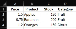
Example: We prepare a range with columns Price, Product, Stock and Category.
2. Decide what you want to find
Identify your lookup value and where you want to return the result.
Example: We will be searching the Product column, and returning the Price.
3. Write the XLOOKUP formula
Click into the cell where you want the result. Type =XLOOKUP( and enter:
- the lookup value (e.g. a cell reference or text in quotes)
- the lookup range (e.g. an area or a named range)
- the return range, of the same size as the lookup range
- the value to return if no match was found
- the match mode
- the search mode
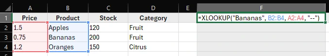
Example: The formula to find the price of the product “Bananas” is =XLOOKUP(“Bananas”, B2:B4, A2:A4, “–“). We use the default values for the match mode and the search mode.
Common errors with LOOKUP
1. I get an #N/A error?
An #N/A error means that Excel or Google Sheets cannot find the value you are searching for. To avoid this, you can either use inexact matching, or wrap your VLOOKUP/HLOOKUP/XLOOKUP formula in an IFERROR or an IFNA function. The XLOOKUP function also has an option to provide a value to return instead of #N/A if no value is found.
Common reasons why this can happen are typos or trailing/leading spaces in your data. Data validation and the TRIM function can help avoid this.
2. There's an #REF! error?
If you encounter a #REF! error, then that means that you are using VLOOKUP or HLOOKUP, and the column- or row-index is outside the range that you specified. For example, if you are returning column 6 from the range A1:D4, then you will see this error. Ensure that your index is within the range you lookup.
3. I get a #VALUE error?
A #VALUE error happens when you use XLOOKUP and the array to search is not compatible with the range of names to return. For example, B2:B5 is not compatible with C2:C4 because XLOOKUP will search the rows of B2:B5 and C2:C4 does not have the same number of rows. To solve this error, ensure that the search and return arrays are of the same shape.
Practical Tips
1. Copy or drag
Copying and dragging formulas in Excel or Google Sheets allows you to look up multiple values easily. However, you should in most cases lock the ranges in your formula with $-signs to keep the ranges fixed.
2. Returning multiple columns with XLOOKUP
You can use XLOOKUP to return several columns or rows at once, by providing a return_range that is several columns (if lookup_array is a column) or several rows (if lookup_array is a row).
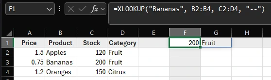
Example: The formula =XLOOKUP(“Bananas”, B2:B4, C2:D4, “–“) returns both the C and D column values for the matching row.
Keep reading
If you found this guide useful, these articles cover related ground:
- The three Excel functions powering the world — VLOOKUP is one of them. See which other two made the list and why they matter.
- Create an ROI Calculator in Excel — A practical walkthrough that puts lookup functions and other formulas to work in a real business model.
- Connect Excel to a SQL Database with Molnify — When your VLOOKUP data grows into thousands of rows, a database backend keeps things fast.
Your VLOOKUP skills are worth more than a spreadsheet
The formulas you just learned can power more than a spreadsheet. Molnify takes your Excel file and turns it into a secure web application that multiple people can use at the same time. Your VLOOKUPs, your formatting, your logic stays exactly as you built it.
You upload the file, add colour to mark which cells are inputs and outputs, and Molnify generates the app. No code, no migration, no rebuilding from scratch. See a full walkthrough or watch the video.
VLOOKUP/HLOOKUP/XLOOKUP FAQ
What is the difference between VLOOKUP and XLOOKUP?
VLOOKUP searches down the first column of a table to find a match and returns a value from a specified column in the same row. XLOOKUP is more flexible — it can search in any direction (up, down, left, right) and doesn’t require counting columns. It also lets you set a custom message if no match is found.
When should I use HLOOKUP instead of VLOOKUP?
Use HLOOKUP when your data is arranged horizontally — that is, when the value you want to match is in the top row, and you want to return a value from a row below. If your data is arranged in columns, VLOOKUP (or XLOOKUP) is usually better.
What is a range lookup?
A range lookup — also called an approximate match — doesn’t look for an exact value. Instead, it scans the first column for the largest value that is less than or equal to what you’re searching for. Put another way, it finds the first value larger than your lookup value and returns the row just above it.
For this to work correctly, the first column of your table must be sorted in ascending order.
Is XLOOKUP better than INDEX and MATCH?
XLOOKUP combines the flexibility of INDEX/MATCH with clearer and more maintainable syntax. However, INDEX/MATCH is compatible with older Excel versions.
LOOKUP in Excel vs Google Sheets
VLOOKUP, HLOOKUP and XLOOKUP all work the same in both Excel and Google Sheets. However, older versions of Excel might not support XLOOKUP.
Google Sheets has XLOOKUP since 2022. Google Sheets’ complete function list is available in its documentation.
Will my VLOOKUP formulas work in a web app?
If you use Molnify to turn your spreadsheet into a web application, yes. Molnify supports over 200 Excel formulas natively, including VLOOKUP and HLOOKUP. Your formulas run exactly the same way in the browser as they do in your spreadsheet.
Can I use LOOKUP functions in a Molnify-powered app?
Yes, you can! Molnify supports VLOOKUP and HLOOKUP. However, for complex lookups or for larger datasets of thousands or even millions of rows, consider using Molnify’s SQL database to power your lookup. See how in our guide on connecting Molnify to SQL.